
 Guillaume Lebedel · · 8 min read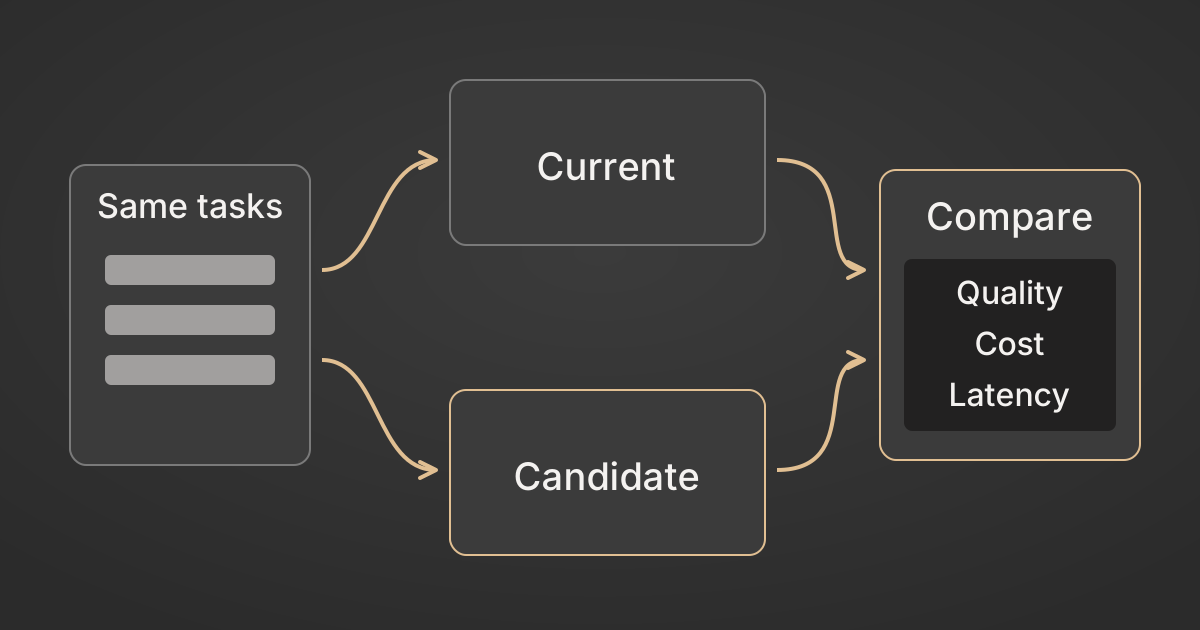
Re-benchmark your agent before a model swap
Table of Contents
Before changing an agent’s model, run the same representative tasks through the current and candidate configurations. Compare total spend per completed task alongside success, latency and human fallback work. This runbook produces that comparison and makes an inconclusive result explicit.
You need saved task inputs, repeatable tool responses, access to usage records and a success rubric. The worked example uses Python 3’s standard library and illustrative records, so it can run without provider credentials or paid model calls.
1. Define completion and freeze the comparison
Write the success criterion before running either model. For a support agent, success might require a draft that uses the right account’s records, states the relevant facts and performs no unauthorized action. Valid JSON or a fluent answer is not enough.
Many production tasks require several model calls. Put a task ID and attempt ID on every call, and keep retries under the original task. Record the model version, prompt version, effort, tool definitions and retry policy.
Freeze the task inputs and relevant tool data. Use recorded reads or a resettable test environment, and simulate writes. Otherwise one run may change the state that the next run sees. Alternate or randomize execution order to reduce time-of-day and provider-load effects on latency.
Keep the first comparison’s prompt and tools fixed. If the candidate needs adaptation, label that as a second configuration and assess it on held-out tasks.
2. Choose paired tasks and repeated trials
A set of 100-300 representative tasks can be an initial screen. It is not automatically enough to resolve a one-percentage-point success difference: that difference amounts to only one to three outcomes before you split into categories.
Sample the traffic mix, including long tasks, tool failures and cases that need human review. Keep a separate set of critical cases even if they are rare. Record category weights so an oversampled difficult category does not silently change the aggregate result.
Run both configurations on each task and repeat stochastic trials. Choose the repetition budget before examining results. Score outputs with the same rubric, preferably without showing the grader which model produced them.
Estimate uncertainty on the paired difference. For example, bootstrap task IDs with replacement, carrying both models and every repeat for each selected task together. Treating repeats as unrelated tasks overstates the effective sample size. Use category-aware resampling and fixed traffic weights when the evaluation is stratified.
If the interval is too wide for your tolerance, the result is inconclusive. More repeated trials help measure model variability; more distinct representative tasks help establish how broadly the result applies.
3. Aggregate spend without dropping failures
Normalize each provider’s usage into disjoint billable categories: uncached input, cache reads, applicable cache writes and output. Apply the relevant rates, including units and retention tiers. Some providers include cached input in total input, so normalize before adding charges.
For each evaluated task run, sum every call and retry before recording the final outcome. Then calculate:
cost per completed task = spend across all task runs / successful task runs
success rate = successful task runs / all task runs
With no successful runs, cost per completion is undefined; report spend and failures directly. When you repeat tasks, each planned repeat is one evaluated task run, while internal retries remain part of that run’s spend.
Keep external tool charges and human fallback cost separate unless you explicitly include them in the cost definition. Also report p95 latency, abstention rate and human minutes. A lower model bill cannot tell you whether the support queue grew.
A runnable example
Save this as compare.py and run python3 compare.py. Each CSV row is one paired trial; each dollar amount includes all model calls and retries for that trial. These illustrative eight pairs cover four tasks with two repeats each. They demonstrate the calculation and are far too small to validate a production migration.
import csv
import io
import random
from collections import defaultdict

records = """task,trial,current_usd,candidate_usd,current_ok,candidate_ok,current_minutes,candidate_minutes
A,1,1.00,0.60,1,1,0,0
A,2,1.00,0.60,1,1,0,0
B,1,1.00,0.60,1,1,0,0
B,2,1.00,0.60,1,1,0,0
C,1,1.00,0.60,1,0,0,4
C,2,1.00,0.60,1,1,0,0
D,1,1.00,0.60,0,0,4,4
D,2,1.00,0.60,0,0,4,4
"""
rows = list(csv.DictReader(io.StringIO(records)))
for model in ("current", "candidate"):
    spend = sum(float(row[f"{model}_usd"]) for row in rows)
    successes = sum(int(row[f"{model}_ok"]) for row in rows)
    minutes = sum(int(row[f"{model}_minutes"]) for row in rows)
    cost = f"${spend / successes:.2f}" if successes else "undefined"
    print(f"{model}: {cost}/completion, "
          f"success={successes / len(rows):.1%}, fallback={minutes} min")

by_task = defaultdict(list)
for row in rows:
    by_task[row["task"]].append(
        int(row["candidate_ok"]) - int(row["current_ok"])
    )
deltas = [sum(values) / len(values) for values in by_task.values()]
rng = random.Random(0)
samples = sorted(
    sum(rng.choices(deltas, k=len(deltas))) / len(deltas)
    for _ in range(10000)
)
low = samples[int(0.025 * (len(samples) - 1))]
high = samples[int(0.975 * (len(samples) - 1))]
print(f"Success delta 95% bootstrap interval: "
      f"{low * 100:.1f} to {high * 100:.1f} pp")
Expected output:
current: $1.33/completion, success=75.0%, fallback=8 min
candidate: $0.96/completion, success=62.5%, fallback=12 min
Success delta 95% bootstrap interval: -37.5 to 0.0 pp
The candidate’s model cost per completion falls 28%, even though it completes fewer runs and adds four minutes of human work. If the predeclared quality tolerance were a one-percentage-point decline, this interval would cross the threshold of −1 point. Hold the migration: the quality result is inconclusive. Inspect task C and collect more representative evidence.
This simple bootstrap assumes equally weighted tasks with the same number of repeats. With only four tasks, its interval is a teaching example, not a reliable production confidence statement. For a real decision, also estimate uncertainty for cost and latency using the same paired task groups; resamples with zero completions need to remain visible as undefined cost ratios.
4. Inspect abstentions and effort before calling a win
An abstention can prevent a wrong answer and still create work for a person. In Artificial Analysis’s GPT-6 evaluation, Sol’s AA-Omniscience hallucination rate fell from 92% to 60%, while questions attempted fell from 99% to 83% and overall accuracy fell from 59% to 54%.
Those metrics use different denominators; a lower hallucination rate is not the same as a higher completion rate. Your success rubric and fallback records should reveal the tradeoff. The example above also shows why model cost per completion alone can miss it.
Effort is another source of misleading comparisons. Anthropic’s Opus 5.5 claim describes lower running cost at default settings, while Artificial Analysis’s maximum-effort evaluation found per-task cost roughly level with Opus 5. Record and test the settings you would deploy. Do not transfer a saving from one configuration into another’s budget.
5. Record a decision and keep the fixtures
Before the run, write down the acceptable quality loss, desired cost change, latency limit and critical failure categories. Define three outcomes:
| Outcome | Decision rule |
|---|---|
| Promote to a limited rollout | Evidence clears all gates, including uncertainty, and critical cases pass |
| Reject the candidate | A critical requirement is breached or evidence supports an unacceptable regression |
| Inconclusive | Uncertainty spans a decision threshold, category coverage is insufficient or fixtures do not represent production |
Review per-category results before the aggregate. A large saving on easy tasks should not hide failures in a business-critical category. During a limited rollout, monitor the same task metrics and retain the previous model configuration for rollback.
Save the fixture set, configuration, usage records, grader output and decision together. Those reusable artifacts make the next model swap quicker to evaluate.
Release and benchmark examples checked against the linked sources on 25 September 2026.